How to vlookup and return multiple values in Excel
From How to vlookup and return multiple values vertically in Excel? (extendoffice.com)
How to vlookup and return multiple values (vertically) in Excel?

Normally, you can use the Vlookup function to get the first corresponding value, but, sometimes, you want to return all matching records based on a specific criterion. This article, I will talk about how to vlookup and return all matching values vertically, horizontally or into one single cell.
Vlookup and return all corresponding values vertically
Vlookup and return all corresponding values vertically
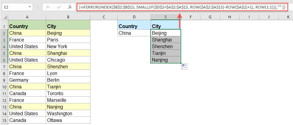
To return all matching values vertically based on a specific criterion, please apply the following array formula:
1. Enter or copy this formula into a blank cell where you want to output the result:
Note: In the above formula, B2:B15 is the column contains the matching record you want to return; A2:A15 is the column contains the criterion; and D2 is the specific criterion that you want to return values based on. Please change them to your need.
2. Then, press Ctrl + Shift + Enter keys together to get the first value, and then drag the fill handle down to get all the corresponding records as you need, see screenshot:

Vlookup and return all corresponding values horizontally
If you want to get the matching values displayed in horizontal order, the below array formula can help you.
1. Enter or copy this formula into a blank cell where you want to output the result:
Note: In the above formula, B2:B15 is the column contains the matching record you want to return; A2:A15 is the column contains the criterion; and D2 is the specific criterion that you want to return values based on. Please change them to your need.
2. Then, press Ctrl + Shift + Enter keys together to get the first value, and then drag the fill handle right to get all the corresponding records as you need, see screenshot:

Vlookup and return all corresponding values into one cell
To vlookup and return all corresponding values into a single cell, you should apply the following array formula.
1. Enter or copy below formula into a blank cell:
Note: In the above formula, B2:B15 is the column contains the matching record you want to return; A2:A15 is the column contains the criterion; and D2 is the specific criterion that you want to return values based on. Please change them to your need.
2. Then, press Ctrl + Shift + Enter keys together to get all matching values into a single cell, see screenshot:

Tips: This formula only applied successfully in Excel 2016 and later versions. If you don’t have Excel 2016, please view here to get it down.

Comments
Post a Comment